Monday, May 13: Handheld GPS

Introduction:

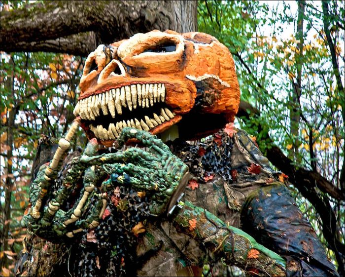
                This semester’s last exercise will be based on digitization of real world features with a handheld GPS unit. For it, we will be returning to the Priory and dividing into groups of three that will navigate the land in order to collect field data from three different categories of information.  This is the same property that has been traversed by the class four times over the course of the semester, and from experience we know that it has a number of trails crisscrossing well over one hundred acres of wooded hills. 

Figure 1: The Priory

               The goal of this project is to prepare and deploy a geodatabase which employs domains and ranges to assist in data collection, then after collecting the data to import the information found into a GIS and display a professional-level map of what was found in the field.  Furthermore, information that was considered of potential importance to the project was determined and collected with the location of material collected in the GPS.  The trio in which I was digitizing data selected benches, erosion, and the invasive species buckthorn to collect and analyze data from.

 Methodology:

                The first task in our final adventure is to develop a geodatabase that can be deployed to a mobile GPS unit for data collection.  For this, the typical steps in developing a geodatabase in ArcMap were followed (as outlines in earlier posts), along with the creation of a point feature class for benches, erosion, and invasive species.  For each, domains were developed and included in the geodatabase in order to improve and speed data collection.  For bench data, the quality or condition of the bench was included (as useable, useable but needs repair, or unusable).  With the invasive species of buckthorn as well as erosion, the amount encountered was included in the data collection as well (low, medium, high).  Finally, a notes field was included to each feature class to provide an outlet that could record any unforeseen but still important or useable data collection.

fig 2: Creating a Domain

fig 3: Setting a domain in a feature class

                After developing these domains, the ArcPad Data Manager Extension was used to import this geodatabase to the chosen GPS unit.  In addition to returning to the Priory for this project, the final installment of our field methods class includes the return of the Trimble Juno handheld GPS unit (fig 4) which was what the database was uploaded to before heading into the field.  This process was simplified by the “Get Data for Arc Pad” wizard, activated by clicking the “Get Data for Arc Pad” button on the ArcPad toolbar (fig 5).  This program helps guide a user through selection of which data to export to the Juno, along with photograph options for feature classes and output options and extraction criteria.

fig 4: the JUNO

                Data collection was a fairly straight forward process:  our group simply set out a path which trekked through the priory following a major foot path and digitized the locations of our selected features as we encountered them.  Being that none of the selected features were continuous, each individual group member decided to collect each feature in the event of problems arising with the data collected by one (or two) of the group members.

figure 5: the ArcPad toolbar
First button with arrow is to deploy to a GPS, button with left arrow is to import from 

Finally, once satisfied with the data collected it was returned to the GIS and prepared into a map that displayed the data collected by feature.  The importing was also done through a wizard accessed from the tool bar called “Get Data from ArcPad” (fig 3).  Esri doesn’t fool around with the names for their tools, which is nice because it makes them easier to use.   After completing the steps outlined by this program (which merely consist of selecting the data to upload onto the computer), the data was successfully imported and manipulated into a useable map.

 Results:

fig 6: the Final Product

The first takeaway that I had from this exercise, and the first bit of advice that I have for any trying to recreate it, is to know your technology.  Twice the technology failed my group in this exercise, first in my attempts to upload my database to a GPS unit that was known to be faulty (unbeknownst to myself), and again when my team member Joey was mysteriously unable to acquire a satellite fix with his Juno unit.  Countless minutes of my life were washed away in a futile effort to do something that would not ultimately be done, and an opportunity to gather data was similarly wasted by the technology failing to work.  I could not help but appreciate the irony that the final project done in this class harkened back to one of the very first lessons imparted on us by professor Hupy: don’t trust technology, if it can fail, it will and often at the worst possible times.  Fortunately, Brandon and I had also been collecting data that would otherwise have been Joey’s domain, and the group successfully completed the task of mapping three different features at the Priory.

Another takeaway would be that the handheld GPS is not always the most accurate data collection unit, especially when the sky is obscured by trees.  While much of the data collected by Brandon and myself matched closely, some simply did not and this combined with the earlier paragraph is a lesson in the limitation of GPS data and a reminder about the importance of knowing how much you are willing to trust the data given to you.

Monday, April 29: High Altitude Balloon Launch

Introduction:

Today’s exercise is the culmination of the previous several weeks spent working on balloon mapping and aerial rigs, etc.  Today, we will fly.  We will soar.  We will launch the University of Wisconsin- Eau Claire into space.  Having finally perfected our camera apparatus and being that the weather appears cooperative, on Friday, April 26 of 2013 the class rigged our space platform to our weather balloon and said our prayers as we floated our helium-powered remote sensor 60,000 feet into the stratosphere.  Hopefully, the camera will parachute safely back to us and we can recover some interesting imagery from our High Altitude Balloon Launch.

 

fig 1: Launch

Methodology:

As can be found in previous posts, this project is something that the Field Methods class has been preparing some time for.  More information can be found in the post for Monday, Feb 11 but I will recap the section that pertains to the HABL.  This activity will take a camera into the upper section of the Earth’s atmosphere, so if we desire to recover any data from the activity we will need to take precautions that combat certain elements of that region of the planet.  Our camera rig will need to

1)      remain attached to the balloon

2)      hold a camera, parachute, and GPS tracking device

3)      deploy the parachute effectively when falling

4)      be light enough that the balloon can rise with it

5)      be stable enough that the camera it contains will capture serviceable imagery

6)      insulate the electronic components enough that the extreme cold, heat, and low pressure of the upper atmosphere does not do any damage to them nor will impact with the earth

7)      be waterproof

  

The rig was based around a Styrofoam outer shell built from a modified tackle container.  A hole was cut in the bottom and plexiglass cover fitted so that the camera could take images through it.  The camera itself was set to take video from this porthole, it was expected that the camera would support an hour of video recording and that the launch would require about forty five minutes to reach its maximum height.  Also included in the rig was a GPS tracking device that Prof. Hupy had effectively rigged to his iPad.  During the launch, this would quickly stop being tracked as its distance from eath’s surface expanded, however it did send out a couple of locations (one every ten minutes to preserve battery life) so that we could see its immediate eastward movement from Eau Claire.  For insulation, some fiberglass and activated (shaken) hothandz hand warmers were used inside the Styrofoam rig once the GPS and camera had been strapped in place.  The top of the box was then taped on with more than enough duct and packing tape.

fig 2: the (rough) general idea for the parachute: let the balloon pop and the parachute should open up as air is forced into the opening under the canvass on the trip down

The Styrofoam camera rig was attached with carbineers to the parachute that would hopefully land the apparatus safely upon the balloon’s popping.  The parachute was then attached to the balloon itself at the center of the canopy, so that it would be held taught as the balloon rose but once the balloon was gone it could catch on the trip back to earth (fig).  The balloon itself was a helium weather balloon which was filled large enough that, as one classmate put it, one could easily roll up and fit a person inside (roughly 8 feet in diameter).  It could have been filled further, but as the balloon rises and the pressure outside of it expands, the gas inside the balloon will not be pushed in as forcefully from the outside atmosphere and the balloon itself will expand.  Obviously, it is undesirable for the balloon to expand beyond failure too quickly, so space was left inside the balloon that the Helium gas could expand while maintaining the buoyancy required to lift the apparatus and parachute through the stratosphere.



fig 3: in the dangerous job of transporting Hydrogen, much care is needed. Good thing we're using Helium.

fig 4: Thank you, professor, for recovering the data!

 The final crucial step in completing a High Altitude Balloon Launch is the recovery of the apparatus itself, accomplished in our case by Professor Hupy and a small cadre of students able to drive to the far side of Clark County where the balloon landed in the canopy of the Wisconsin Woods.  The balloon had to land before the GPS unit was sending its signal to the iPad, and Hupy had to saw some branches in order to get at the balloon, but the rig was successfully recovered and with it, the data (fig 4).

Results:

the Curvature of the Earth

The ultimate result was a sweet video of the earth!  The parachute was successful, and out apparatus was found safely dangling thirty feet up a tree in Clark county, just under 80 miles from the launch site.  If you did not know, this is an exciting accomplishment in and of itself.  Several images were collected from the video (given below) and nearing the top of the ascent, the camera apparatus began swaying enough to clearly show the curvature of the atmosphere.  The earth is ROUND, people!!!  More could be done in further projects by attaching some IR cameras to the rig, I personally would like to be able to collect some imagery that would fall under the Landsat 7 band 6 range of data (heat) or perhaps do a night launch and see the lights from the night sky.  Another addition that should have been considered would be an altimeter that recorded the altitude of the apparatus over time, this way we could have an easy tool to determine the height of each image.

the mighty Chippewa River from high above.

Monday, April 22: Balloon Mapping II, Results.

Results:

                This week’s activity rolled out much more easily than last week’s.  The first balloon launch had a number of issues, not the least of which was the weather.  When taking aerial imagery from a lighter-than-air craft, it is obviously quite beneficial to have stable air conditions.  The wind during the first launch provided the class with some interesting images, however not many that were particularly useful.  Mosaicking works far better with less oblique imagery: the edges work out much better that way.  The more oblique an image is, the more distortion is introduced.  Fortunately, throughout the entire first batch of photographs we were able to pull enough to build a workable mosaic of the area that was walked.  This might be taken to indicate that even with conditions of moderate wind; a slow enough walk-through the area of interest can yield workable results.  Walking speed does not however remedy the problem of getting the tether tangled in local features like buildings or trees introduced by wind… in fact if the project had been completed quicker Bessie may never have taken off over the river.  On that note, while waterproofing may have seemed a luxury at the time I would definitely spend the extra few dollars and minutes next time to ensure that my data is that much safer should trouble arise (or fall).

                When it comes to mosaicking images together, MapKnitter does an okay job, I have to say my expectations were quite low for this free software and I was thoroughly impressed.  It was relatively easy to use, and it’s completely free.  It does have some disadvantages though.  It lacks some functionality present in the more advanced programs offered to the class (Arc and Imagine), and even the best images that I saw mapknitted by classmates don’t quite equal the seamlessness of the images provided by ESRI and ERDAS.

                Speaking of, my group’s final section was produced in ESRI ArcMap.  Georeferencing took a very, very long time in order to get all of those sidewalks to stack well together.

Discussion:

                I can’t believe the amount of work done by half the class… thank you especially amy and bea. Next time, more responsibility needs to be taken by someone to ensure that the project is completed start to finish. …

Monday, April 15: Balloon Mapping II, Methods

Introduction:

In early February, I posted about the early stages in perparing for a method of collecting aerial imagery using helium balloons known as Balloon Mapping. Now, for the past two weeks the class has been making good on the first half of that project: the low-altitude ballon launch has come to fruition. On the 1st and 8th of April, the launched our noble apparatus and towed it around the campus here at the University of Wisconsin -- Eau Claire as it collected thousands of aerial images from which to develop a single image of campus tied to defined geographic reference points. The following is an account of the methodology of our launch and image processing, as well as what was learned in the class's two launches.

 The goal for this section of the project is to develop a high-quality, georeferenced aerial image of campus.  We will require the helium balloon, an effective compartment to house and protect a digital camera inside, and the software to combine disparate images into a single unit.  This week’s blog post will describe the methods used to develop the rig, collect images, and process what was collected.

  

Methodology:
    Launch 1:
          The first launch was conducted on Monday, April 1^st.  April 1^st in Eau Claire, WI was windy, to say the least. Naturally, the wind was highest during the period from 3 to 6 p.m. which was exactly when it was decided to launch the aerial rig.  Noticing wind speeds around 15 mph and gusts in excess of 25mph, it was decided to use the more substantial platforms to house the digital camera today; so the HABL rig was attached to the helium balloon instead of the Low-Altitude rigs developed for the project.

 

figure 1: wunderground historical weather data for Eau Claire, WI on Apr 1. Note the wind gusts around 4 PM.

The HABL provided certain advantages over the other aerial mapping platforms: it was more insulated, painted with hydrophobic material for waterproofing and heavier which it was reasoned would provide more stability in the wind.  Its design was based around a Styrofoam bait container, the type used in fishing which would prove fatefully ironic. Perhaps most importantly, it was heavier and therefore (in theory) less susceptible to the prevailing winds, however the end results of this project indicate that the added weight was inadequate in this case. 

         
           Bessie, as the big red weather balloon came to be called, was attached to 400 meters of rope in addition to the camera platform and released into the air while attached to a ground crew whose duty was to guide the balloon around campus (and around obstacles on campus, such as light poles, buildings etc.).  In the wind, however, Bessie's actual distance from the ground was significantly reduced from 400m because she was pushed some distance away from the ground control crew in the breeze.  It was attempted to find her precise height using the radar distance finder (see distance azimuth exercise) but this attempt met poor results.  The camera rig was tossed around rather harshly in the turbulence, which had the side effect of providing some nice oblique images of campus caused some concern for those on the ground.  Regardless, the exercise continued as scheduled and the ground crew guided Bessie through the area until she broke free and made for the horizon somewhere over the bridge connecting campus across the Chippewa River.  Fortunately, she was kind enough to drop her payload in the river before lifting off, and being waterproof the images retrieved from the day were quite usable after the rig was fished from the River by Professor Hupy.


     Launch 2:
           Monday the 8^th provided far clearer weather than the week prior, and as such it was decided that a less weight-intensive payload could be attached to the second balloon (named Bertha).  The old Low-Altitude, bottle-based design for the rig was improved by Stacey’s addition of an old arrow whose fletching was augmented with cardstock to stabilize the rig in the air and keep it from spinning much in the wind this time.
       

          The rig was launched to a height of 550 meters and guided through campus much like it had been one week prior, but today the balloon was recovered as well as the imagery.  Because of the good weather conditions, the balloon was taken over significantly more territory on this occasion than earlier.



     Processing:
            The class was allowed to use any combination of three programs to mosaic the images from each rig into a pair of georeferenced orthophotographs of campus: ArcMap, Imagine, and MapKnitter.  Some students used the online services of MapKnitter, but I decided to use ArcMap, having mosaicked orthophotos in Imagine before and feeling some trepidation about the quality of Mapknitter’s abilities to provide a seamless image.  Before Images can be mosaicked however, they must be georeferenced to locations on the earth.
         
            The first task is to select the images to be used for processing from the camera.  When looking for a good image, one looks for an image that is taken as close to directly overhead as possible: oblique images are not very useful for mosaicking.  In the first set of images, this restriction made selecting appropriate images difficult as many of them were very oblique indeed.  The second set of images was difficult to sift through simply because there were so many usable images, which is a good problem to have I suppose.

           After the enough images to cover the area of interest have been selected, they need to be georeferenced.  One does not simply piece each individual image together and call it done: the pixels in the image need to be tied to coordinates in reality using georefrencing.  To do this, several “control points” in the image are selected which are readily identifiable and relatively stationary such as lamp posts, building corners, or road edges.  These points in the image are then “tied” to the geographic coordinates of that point in reality; this can be done in several ways.

One way is to use another image, which is already georeferenced, on which to overlay the new image being referenced.  The points in the new image are selected, and then related to the points in the original image in order to warp the new image into an appropriate approximation of reality.  Another possibility is to use GPS or Surveying in order to physically collect each point in the field, and use these points to connect to the image being georeferenced.  For both sets of images, I used a georeferenced basemap to tie my GCP’s to, but for the second set of images a group of students also set out to collect GCP’s using GPS equipment.

In Arc, this requires the Georeferencing toolbar.  First, a dataset with spatial reference is opened, and the new image is imported on top of it.  Not having any spatial information, the new image will not be displayed with the currently open map and so must be added to the display by using the “fit to display” tool on the georeferencing toolbar.  Then, the rotate, shift and scale tools are used to roughly position the image where it belongs in relation to the control points of the map.  Then, the control points on the map are selected individually and connected to the control points of the reference image.  Finally, a transformation is applied to the raster which warps the image to best fit the changes in each point.  Most of the images I mosaicked used 2^nd-order polynomial transformation.

            Finally, once all of the images are selected and georeferenced, they need to be mosaicked together into a single orthophoto.  In my case, this is accomplished by using the mosaic to new raster tool in ArcMap, which creates a fresh new image from my multiple component images.  For the first set of images, I used eight photographs to create a rough mosaic of campus.  For the second set of images, there were so many photographs covering so much of campus that the class divided the area into six sections and worked on each section in groups of three.  Then the class uploaded each section into a class geodatabase to be finally pulled together in and a single, high-quality image of campus from the class will have been made.

Monday, March 25: The Navigatorial Competition and a Comparison of

Introduction:
 

This week's activity is best described as the culmination of the previous month's work. Each team of three will be provided with both the land nav maps and the GPS units, and will be tasked with finding all fifteen points in the course. To add a level of urgency to the exercise, all six of our groups will be in competition for the fastest navigation in the class. The fastest (or most complete) group in three hours will be declared winner; what exactly they win is as yet uncertain but it must surely be something pleasant. Most likely, the answer is simply 'not getting shot,' because as a final measure to complicate our traversal of the Priory is the inclusion of paintball guns. The ultimate goal of this task is to see how well our navigation skills will hold under duress, hopefully we shall pass.

 

Study Area:

For March, the terrain around the Priory has not altered much since our first excursion on the 11th. This is at once both a good and a bad thing: in particular the persistent snow cover continues to impede our ability to make use of the aerial imagery and digital elevation models in our land navs. In addition, when multiplied over the size of the entire course, the snow which at places remained waist high was a tremendous burden to movement. With this in mind, Professor Hupy decided to offer snowshoes (fig 1) to the class for this exercise.

 

I did not wear the snowshoes, but from a distance they looked a good deal like these.

In my estimation, choosing snowshoes would improve my ability to trek over a distance but could be an extra burden in a fight, restricting my maneuverability in the sometimes thick niches of the Wisconsin Woods which can make for wonderful mock-ambushes. I chose to forgo the snowshoes on today’s journey.

A few changes have been made to the course for this week’s activity from our last encounter with the Priory.  As mentioned earlier, this week we are expected to (or striving to) visit each checkpoint on the map.  Furthermore, because of the similarity that paintball markers bear to real weapons and the proximity of the Priory and Interstate 94 to our activity, Joe has designated several areas as off-limits to the navigation.  There will be no shortcuts or firefights across the Nature Academy’s Lawn. These areas have been designated on both our aerial and topographic maps (fig. 2 and 3 below).

fig. 2: the final aerial

 

fig. 3: the final topo

 

Methodology:

            The final maps created for this activity are above, including both the off-limits zones and each of the points that should be navigated to during the afternoon.  The groups are allowed to make use of all, or none, of the previously learned tools in our belts: the compass, GPS, and of course maps are all available and acceptable.

fig. 4: the Garmin Etrex H

The data collection this week will be done with Garmin Etrex Handheld GPS’s again (fig 4), taking a continuous tracklog at 30s intervals.  We will also have to input each waypoint from the course into the GPS as a waypoint.  The Etrex are set to record position in UTM coordinates (zone 15N), and will be used for navigation as well as data collection as participants are given the coordinates for each point at the outset of the exercise.  As a final quality assurance / quality control measure (safeguard against tomfoolery), each team will again receive a punch card which has unique punches to be received at each individual navigation point.  

            After the event is finished, each group will again export their tracklog and waypoint data from their individual GPS into the GIS using the DNR_GPS program.  After downloading the GPS information using this program (fig 5), the data will then be compiled by the professor to make available to the class through the GIS on UW-Eau Claire’s network.  The final stage of this project will be to look at the data in ArcMap and analyze what each team did, and see how well it worked.

    

fig 5: DNR GPS, pre-loading. The path to download is GPS>>Connect to GPS then Track (or Waypoint) >> Download.
Connect GPS to computer before attempting.

Discussion:

          The final data is not altogether surprising.  The final map is figure six below, and by looking closely at it one can see that groups branched off most in the beginning (start was just north of the Priory) and in the middle of the map especially closest the interstate where compressed againt a hill  the groups clustered along a single path almost exclusively.  Some points of conflict can be seen clearly, in a few areas it appears as though a conflict may hav forced a group or so to shift course.  An example of this can be found halfway between points 1A and 2; or directly north of point 5B just south of the restricted zone.

fig 6: the final Aerial Map with Each Group's Tracklog.

          Each point was visited, but no group visited each point.  Suprising to me was that point 4 got hit by each group, while it was extremely remote and difficult to find. On the other hand, point 5A was easy to reach because of the flat terrain and nice forest cover that kept the snow lower, but it hardly recieved any visitors by comparison to many other points. 


Conclusion:

With regards to the terrain itself, it would be a lie to say that I did not wish that I had taken the snowshoes by the end of the trek. While I stand by my previous assertion that snowshoes can be an impediment during a fight, I do not think that the slight loss of ability on a small number of occurrences warrants the massive amount of energy exerted unnecessarily fighting the elements.  Watching my colleagues glide across the snow after a fight, I determined that the snowshoe/no snowshoe issue is best summed up in fig. below.  I would conclude that snowshoes were beneficial to those that wore them.

Snowshoes

Noshoes

            Personally I found that I prefer to trust the land maps to the GPS units.  There are advantages and disadvantages to each, but in this situation I found that using the maps to navigate with provided data that was simply not available through the Etrex.  That aside, my group spent much of its time working forward with our noses half buried in the diminutive screen of the handheld GPS in an effort to stay on course.

There is something to be said for knowing one’s exact location in relation to a goal, and if lost (as we would have been on several occasions after a particular battle or two) the GPS gives the immediate position of the beholder.  On the other hand, valuable time could have been wasted trying to conclude our position on a map.  Of course, maps never run out of batteries which is a situation that my GPS appeared to be nearing a mere three hours into the activity.  Ultimately, the ideal navigation scenario for me would include both a GPS and a map.

    

Monday, February 25: Land Navigation Maps

Introduction:

     This week is going to be a short post; much as how on the 18th I provided only the first half of an exercise (which has yet to be completed, we'll get there eventually!) this week's project was more preparation and less completion.  The ultimate goal for this week is to prepare for next Monday when we will be working in the field, conducting a survey of the "Children's Nature Academy," also known as the Priory and a recent acquisition of the University's.  The property contains over one hundred acres of former monastery lands: three buildings containing over 80,000 square feet, and plenty of wooded lands just past the outskirts of Eau Claire.  In preparation for this survey, we are going to do two things: find our individual pace count and develop a navigation map.  This week, we will be grouped in threes: my partners are Joey and Brandon (both of whom keeps a very nice blog as well, by the way).

fig 1  St. Bede's upon acquisition

Methodology:

     The first item to get out of the way is the pace count.  Professor Hupy informs us that we will be needing this count for next week, so some dead reckoning is to be expected in our navigation.  The entire class paced out 100 meters on flat terrain four times to determine how many paces each individual has in that distance (this is a standard pace count).  One pace is every other step, starting on the left foot every right step would be counted.  These steps are supposed to be casual, like one would do when hiking.  My first set was 67 paces, followed by three sets of 61 paces so I'm going to call my count 61.  When in the field, I will have to estimate (or guesstimate) how the terrian is affecting my step size to figure what difference it may make in my pace count and keep me from getting lost in a one hundred acre wood.  For such a small and simple task, this step is perhaps more important to do correctly than the making of the map; a bad map may still be workable on a small scale if you are able to calibrate distance correctly, but the opposite is not true.  If I get lost, I intend on using the serene sounds of the nearby interstate to guide me towards civilization, but if there's no traffic and I get lost then there will be a problem.



fig 2  The UWEC Campus, the Priory is in the lower left, quite away from the rest of campus.



fig 4 What happens to those who do NOT know
how far they've travelled

fig 3 What happens to those who know
how far they've travelled

 

     With pace counts in hand, it is time to develop a navigation map that will be used in the field.  A good deal of data was provided by the Professor Hupy and our talented Geospatial Facilitator Martin Goettl: aerial imagery of the area in both color and black and white, topographic data contour AutoCADs at both 2m and 5m intervals, a DEM (see my second post), an actual USGS topo map (Digital Raster Graphic, DRG), and boundaries for both the navigation area and the point area.  The topographic countours were developed from a the DEM which was downloaded from the USGS seamless server, and the DRG image came from the same place.  The ramaining data was developed for a UWEC survey.
     Our final product needs to be a pair of 11x17 maps projected into UTM (Zone 15N) that are going to guide our navigation through the wilderness with a grid overlay; we are free to include whatever data we feel whatever will be useful.  The maps also must contain the data sources and projections being used.  For a project like this, it was decided that UTM would be the most valueable projection because of the low distortion although a county system might have been more precise, because UTM coordinates are easy to understand and universal.  Unprojected coordinate systems (latitude-longitude) are So the first trick is to project all of our data into UTM as to ensure that it matches for the map.
     Most of the data was already in UTM, however the AutoCad topographic contours at the 2-m interval were neither in UTM nor was their projection defined when we recieved the data, so when ArcMap attempted to lay it on top of the other datasets already laid out it was unsuccesful (figs 5 and 6).  Thus began the process of discovery that can be working with a data set sans metadata.



figs 5+6 or Projection: you're doing it wrong. The top image is the 2m contour, the bottom is our USGS topo with 5ft contours in red. Notice the highlighted coordinates, and how they don't match by roughtly forty degrees longitude. This will have to be remedied.

     To solve this problem, we needed to determine the original projection of the data and define it so that it could be projected by the software.  There are several ways to accomplish this task, myself and at least one other classmate attempted to guess the appropriate definition a few times until we got lucky, which actually worked when Beatriz tried the Wisconsin Tranverse Mercator and our contours fell right into place.   This makes sense, since WTM is the state system projection for Wisconsin, a good choice for USGS topographical data. Of course, guesswork is never professional, so although the data looks good and may work for personal purposes it is still useless until it can be shown that this is indeed the projection that the data was imported in.  This can be solved by either re-loading the data ourselves or asking the data provider(s), in this case USGS or Martin.  Martin, having an office across the hall and being immediately available, was willing to find the original download and found that in fact the data did arrive in Wisconsin TM.

fig 7 or Projection: you're doing it right. Notice how all those lovely blue 2-ft contours line up with the topographic raster? You may need to expand the image. Also, does this map seem busy to you?

     Now that all of the data is in one projection, all that remains to accomplish this week is a little cartography!  Being that we get to use both the front and back of our paper for our maps, our group decided it would be wise to use one map that would be easy to mark as we comducted our survey and one map that showed the terrain in more detail.  The main concerns with creating each map were 1) can we use it to navigate and 2) can we use it to navigate.  The maps need to be readable and not too busy or cluttered to use.  The maps also need to give an adequate idea of the terrain at a given point, and the best maps will balance both.  Fortunately, the ability to have two maps sidesteps the problem somewhat by allowing us to split the information across two maps.
     I created a pair of maps for the excersize, the first was a combination of the color aerial photograph and the DEM (fig 8).  I chose the color aerial instead of the black and white one because it was taken in the autumn and the difference between evergreen and deciduous forest is very clear on it when compared with the black and white.  The digital elevation model was layered underneath a 25% transperent aerial, both rasters had the contrast beefed up 20% as to be more defined.  I could not decide whether to add the 2m contours, because the DEM still did not give a well enough defined idea of slope over the study area for my taste but adding it made the map far too busy and the 5m contour was not useful at all in this regard becasue the spacing is higher than I like.  I settled on adding it but clipped them to the area of interest and turned on the transperency so that the contours don't overwhelm the aerial and DEM.  Overlaying the entire output is a grid of the UTM coordinates at 50 meter intervals to assist with navigation.  I also added a single full color aerial.

fig 8: My Aerial Map. 









     I also created a much simpler map of just the contours with an extremely light DEM underneath for a tiny bit of added clarity. This map is pretty straightforaward (fig 9), I must give credit to Joey for the format of the legend, North Arrow, scale bar etc. as he had already completed his map by this time and I both liked the sharpness of his layout and I wanted to acheive consistency if we were to print maps from different group members.  To make it look nice.

fig 9: My Contour Map

Discussion:

     In the end, our group sent in one aerial image and one 2ft contour map with a light DEM in the background.  The grids we used were at_____ intervals... more soon...like an image of what we sent in...

Monday, February 18: Distance-Azimuth Survey

Introduction:

     Professor Hupy designed this lab to both further our understanding of field methods and (of course) improve out ability to provide low-tech solutions when "in a pinch" high-tech plans fall through.  In it, we will use the distance-azimuth method of surveying to plot points of interest (of our choosing) in a quarter hectare (25 sq. meters, also of our choosing).  In teams of two, we will be using two methods to survey our points; both sets of data collected will be distance-azimuth however they will be collected using two sets of instruments.  The first data set is the combination of a compass and a radio-based range finder which is standing in for the rather unwieldy, if sometimes necessary, tape measure.  The second data set will be collected with a laser rangefinder.

fig. 1 We chose the worst time of day to go outside.
courtesy wunderground.

      Our pair paired with another pair to more efficiently split the workload: with four total members we could collect our data using both methods for each point at one time thereby cutting down on the time required in the bitter cold that was Monday the 18th, circa 4-6 PM.  By the time we were wrapping up the lab, it was 15 degrees with windchill, gusts of up to 20 mph, and snowing, not that we minded (fig. 1). 


What we felt we were doing



What we actually were doing.
Say hi to Joey, he's the one in the middle.

 
     After collecting our data we will import both sets into a GIS and overlay the data sets with a base aerial of the area covered to assess the success or failure of our endeavor. Ideally, the points surveyed with both systems will line up accurately with the aerial.  We selected the backyard area of a residence hall on campus (the area bordering both Horan and Governor's, for those curious) which seemed a good choice because of the myriad trees in the region, sprinkled with a smattering of other objects such as benches and disc golf holes to map.


Methodology:

     So distance-azimuth surveys are quite simple.  The surveyor stands on a known point, and calculates the distance and the angle to the desired survey points.  Then, inside, the surveyor can use simple geometery to determine the location of the survey points using their relationship to the known point.  Therefore, it is integral that an accurate calculation of angle can be found; the budding surveyor must have a working understanding of magnetic declination.  Because of variations in the earth's molten metal core (of which I have only the most rudimentary understanding), magnetic north constantly shifts around true north.  As magnetic compasses point toward this magnetic north, and as good geographers we want our data to be accurate against the standard true north (pole), we must calculate the angular differential between true north and magnetic north from our location on the earth.

fig 4 Magnetic Declination, courtesy NOAA.

     Luckily for we Wisconsinite compass users, this declination is rather small in the area (see fig 4 above, the line of no declination ran just west of us in 2010).  The exact declination for any loaction at any time on earth is conveniently provided free to the public by the wonderful folks at NOAA's geophysical data center with this magnificent declination calculator.  The declination at the time of our data collection was determined to be 58' W, which means that for true accuracy in collecting our azimuth the laser rangefinder must be calibrated and the compass data must be rotated that far west.
     Understanding this, we calibrated our tools and set out to collect our data.  One team member would walk to each individual point with one radio reciever/transmitter and another would stand at the reference point with the other radio transmitter, which would use the radio waves to determine distance between the two points.  The individual at the reference point with this transmitter would also use a compass to determine the azimuth to the point being surveyed.  Another person would use a TruPulse 360 Laser Rangefinder (fig 5) to simultaneously determine both azimuth and distance to the survey point, while the fourth person took down the data.




fig 5 TruPulse "Laser" rangefinders

fig 6 How the Laser Range Finders will look in the future.

     Unfortunately, we found a few issues with our selected hectare which will be discussed later, but eventually 32 unique data points were collected using both methods.  These points were then turned into an excel file (fig 7).  A reference point was determined by using georeferenced aerial imagery and added to this file, which was then imported to our ArcInfo geodatabase.  In our case, I decided to use decimal degrees because it can be used by the computer and  while I can project the data later if needed, doing so now is not important for the purposes of this excersize.  This reference point was determined to be -91.50696 decimal degrees East, 44.79873 decimal degrees North.  Also, with each point we collected attribute data to describe what point we were collecting, for example if a point was a tree or a post or table etc, so that we can more effectively match our data to an aerial later.

     The tables were run through the Bearing Distance to Line tool, and then the Feature Vertices to Line tool provided with the GIS (under Data Management, then Features).  A nice data flow model (fig 7) for this process can be found on stackexchange, along with an explanation of the process.  Finally an unprojected aerial Basemap was added so that we could compare the accuracy of our data to a previouisly georeferenced image.  The final product is figure 9 below, I digitized some goal points for reference.  Compass and radio points are in blue, data collected by laser is in red. Unfortunately, the data do not line up especially well.  For example, point data with a more easterly azimuth were consistently farther off than other points, but more on that below.


fig 8 Bearing Distance to Line with the end Points.

fig 9 The final product, with some reference points in purple.

 

Discussion:

     As you can see, not only did the data collected with the two methods not match with each other, they didn't match with the terrain.  Several factors could be at play in this discrepancy: the most problematic is that some of our points lied behind other points (trees) and could not be surveyed from our reference point.  Adding a second or third reference point would probably have alleviated this problem.  Being cold and windy, and since two team members were operating without gloves, there was also a decent incentive not to collect the same data point more than needed, therefore  a few discrepancies could be attributed to user error or quick work.  Far more prevalent by the look of the map, the east half of the laser data have consistently more extreme azimuths.  It is possible that the building that we stood in the shadow of interfered with the function of the magnetic equipment used, because obviously we didn't survey our points through the corner of Horan Hall.
     Unfortunately, the spatial and temporal resolution of the image that we are comparing our data to is not very appropriate either.  For starters, in winter those trees look a lot differently than they do in summertime. One of the points surveyed was an unusually large snow pile, which of course would look more different still in the summer.  Some of the smaller features that we collected are also impossible to see, either because the resolution is too small or because they are covered by foilage.  Our quarter hectare was also too small to collect as many points as we wanted: the goal was fifty but even if we could have included the objects hiding behind each other we still wouldn't have managed that many points of interest.  And we cheated by both surveying outside of our hectare and by using fluffy points of interest, such as snow piles.
     Altogether, I am still rather pleased with our end result. I am disappointed in the lack of accuracy, however our radar/compass data was consistently within a few meters of our goal points, which is surprising given the difficulty which the radar tool would occaisionally operate with.  I would certainly have preferred to use a total station for this job.  I would have have more confidence in the preciseness and the reliability of my data, plus I could remove the step of trying to locate myself on an aerial photograph after having already collected my data.  However, by comparison I have to admit there isn't much involved in this process: one handheld tool and a recording device are all that is required to survey the type of information that we were collecting.  I like to travel light.

Monday, February 11: Balloon Mapping I

Introduction:

     This week we spent the class period developing separate apparati for two upcoming mapping projects: one for low-altitude mapping and one for a high altitude balloon launch (HABL).  Professor Hupy describes this project as 'like Apollo 13" in that we were provided with a finite assortment of materials from which to construct rigs to which we will affix digital cameras (and GPS's) that are to act as remote sensors.  The only difference is that in Apollo 13, the folks working on adapting air filters were the best and brightest engineers of a generation and in this case, two dozen undergraduate geographers are trying to send sensitive digital equipment into space and get it back in workable condition (its still not a life or death situation though).  The low-altitude balloon will be held onto by guide wires and taken through campus while a GPS tracks the location of each shot.  After collecting our images, if all goes well, we intend on patching the images retrieved together and generating some nice maps!  But more on that later, for now we need to focus on getting the images!
     As the instructions that we encountered while trying to prepare for this launch over the internet were found to be perfunctory at best,  the end goal of this week's blog is to provide detailed information on how we developed both the low-altitude module and the space module.  This way, the readers will be left with an exact account of what to do (or not to do) when trying to collect images from helium balloons launched into space.


Methods:
     Let me preface this discussion of our methods by stating that this is not a good project for young children: we did use exacto-knives, a leatherman, and a hot knife.  If you and your kids are embarking on the noble endeavor of sending some legos into space, be sure that a responsible person is on hand to do the slightly dangerous aspects themselves.
     Now, the first determination that needs to be made in developing our rigs is what we need the rig to do.  In the case of the High Altitude balloon launch, we need to have a rig that:
     - Can be attached to our helium weather balloon
     - Is light weight
     - Is stable and won't spin uncontrollably in the breezy upper atmosphere.
     - Insulates a digital camera from both physical damage and the elemental cold of the mesosphere, but still allows for the camera to take quality images on the flight.
     - Insulates and protects a GPS unit that can be used to track the end location of our rig
     - Carries and effectively deploys a parachute

The Low Altitude rig must:
     - Still be attached to a helium balloon and still be stable
     - No parachute or thermal insulation is necessary
     - Be attached to guide wires

     Fortunately, our instructor provided a rather large bundle of usable equipment, from which we selected for our launch:
     ~seven pairs of hand warmers
     ~three two-litre soda bottles (empty)
     ~Digital Cameras: TYPE Cameras will be unsing continuous shot mode instead of video as to preserve both image quality and data space limitations.  As such, we will have to rig our cameras with something to hold the trigger down.
     ~GPS/GoPro
     ~Some 1" thick styrofoam insulation
     ~One Styrofoam bait container
     ~Strong rubber bands
     ~Bleach bottle (empty)
     ~Zip ties
     ~Small Carbineers
     ~Two Weather balloons, and a helium tank provided through the University.

     Exacto knives, a small pocket knife, packing tape, and an electric hot knife (insulation cutter) were also used in the construction of our rigs.  Before any consturction takes place, an integral step in the process of developing these balloon-powered craft is identifying the weight capacity of the balloon and the expected weight of the rig.  To that end, several students diligently weighed the components of our craft as well as the final products of the high-altitude module.  Fig 1 is an snapshot of that data in MS Excel.  This is an especially important aspect of the High Altitude Launch, because the goal is to get our camera as far from the surface of the earth as possible while still having it return to us.

Fig 1: Our weight data

Low Altitude Aerial Launch:
     We garnered two seperate attempts at developing a low-altitude model, one unnamed devce (fig 2, 3) and one known as The Hindenburg (fig 4,5).  The constuction of the as-yet unnamed module
consisted of removing the bottom from the bleach container and affixing the camera to the indide with some string.  A rubber binder and pencil eraser were used to hold down the capture button on the camera; plastic wings were fashioned from the bottom of the recepticle to keep the device from spinning in the air, and attached with packing tape as seen in fig 4. The Hindenburg was formed from a two-liter bottle with the camera attached to the side with zip ties. A hole was cut from the opposing side to allow for clear images.  Both modules used string to attach them to the balloon, the unnamed module used the string attached to the container itself and the Hindenburg attached the string to some zipties strung through punchutes made at the oblong ends of the bottle.

High Altitude Balloon Launch:
     The High altitude Module is based around a strofoam minnow container with a hole in the bottom where the camera lens will poke through. COVER The camera is affixed to teh inside with string pulled through the sides of the container, and insulated by seven pairs of hand warmers.  Additionally, a styrofoam cover was cut with the hotknife to help insulate the package further and secure the hand warmers in place against the camera. It will be attached to the ballon by yarn pulled through the sides of the container near the top. Parachute?

Discussion:
    Hopefully we have provided an adequate representation of how we developed our modules. I will be updating this blog post with any modifications made before the launch of each module so that you, the internet-scouring public, can fully take our observations to heart and learn from our experience.  I also notice that we did not take exact measurements as to the dimensions of our models, and I will try to get some before we launch.  As I mentioned abover, the end goal of this batch of posts is to provide better instruction on how to develop modules for both Low-Altitude and (especially) HABL rigs than what we ourselves were able to find.  Now you have our instructions, but it won't be until next week when we get to find out how well or unwell our attmpts worked.

Monday, February 4: Sandbox Mapping

Introduction

                This week, we are extending upon last week’s lessons by first digitizing our original findings.  After we have created some three-dimensional surfaces which try to convey our original data, we will determine how our original approach could be improved.  Using these determinations, we will embark on another survey and develop a second surface, which will be an improvement over the first if not in the quality of the model than at least in the methods used to arrive at it.  Ultimately, our group will have developed two sets of five Digital Elevation Models in an attempt to accurately portray our hand-built "sandbox" surfaces.

Methodology

                The first task of the week is the digitization of last week’s data into what’s called a Digital Terrain Model (DTM).  The immediate problem that we ran into was that the excel table of our data was formatted in the same fashion as our original data collection (image 3 last week): a table where y values are tabulated along the side and x values along the top, so that each point on the table was neighboring point that it would neighbor on the landscape (image12).  This is not useful to the GIS, and so task one was reformatting the table to x,y,z coordinates (image 2).

Figure 1: Our original data table.

Figure 2: Our second data table.

                With useable data, five surfaces that display elevation were developed in the GIS.  First, the x,y data was imported and then converted into a point shapefile (image3).  From that, four surfaces were created with the raster interpolation tools in ARCMap using spline, natural neighbor, kriging, and inverse distance weight (IDW) interpolation.  Also, a TIN was made.  The five rasters are displayed below in ARCMap, along with a brief overview of the meaning of each method.

IDW 1 

IDW 2

Inverse Distance Weighted or IDW interpolation is a deterministic tool which determines each cell's value by finding the average of nearby cells' values.  Closer cells are 'weighted' in this determination, making near cell values  stronger determinants of an individual cell's value than more distant cells' values.  The ultimate value of the cell in question is the value for that cell which minimizes the root mean square prediction error.



Kriging 1

Kriging 2

 Kriging is a geostatistical interpolation method that uses statistical relationships between values in the determining of each interpolated cell value. In addition to considering the data given, this model uses spatial autocorrelation semivariograms to determine which values are factored into the interpolation of each point.  Simply put, kriging determines weight by looking at each value's relationship to other values in addition to their relationships to the value being found.  For our model, we determined that ordinary kriging with a spherical semivriogram would be most appropriate, as there is no external variable we expect to bias our data in terms of elevation that can be defined by an equation and autocorrelation of elevation decreases substantially with distance.




Natural Neighbor 2

Natural Neighbor 1

        

Natural Neighbor interpolation works by  creating two Voronoi diagrams from the dataset for each cell: one using only nearest data points and one using the cell as an additional point. It then weights each nearest value by the percentage of that value's Voronoi polygon which is overlayed with the interpolated value's polygon.  Simply put, natural neighbor works by weighting each point not only by how close it is, but also how close it is to other points in the same direction from the cell being determined.  Doing this 

Spline 1

Spline 2

   Spline Interpolation develops a smooth mathematical curved plane, the function of which fits each input data point perfectly and therefore produces a continuous surface devoid of artifacts.  It usually does better with surfaces that don't contain coarse variation than with regions of varied elevation, because this model will be warped by concentrated variations in input points.

TIN 1

TIN 2

       Triangular Irregular Netwroks (TINs) are simply digital triangles drawn between nearest data points. Which points are connected by the edge of a triangle are determined such that no vertex lies inside the polygon of another triangle. 

                 Once the rasters were complete, a we determined the most effective interpolation methods for our data to be Kriging and Spline.  3D Elevation models were developed for the five models by importing the rasters (or TINs) into ArcScene and setting the base height to the surface of the elevation values assigned each cell.  After playing around with a little symbology, what we ended up with for our Spline and Kriging models can be seen below. 

Spline

Kriging

Conclusions

                 In my opinion, the Kriging model best represents our data of the five DEMs which we developed. It is the only model which allowed for the mesa which I had hoped to digitize which was surprising to me (in the upper left region you will notice a brown hump with a somewhat flat top). It also contained the best ridge between the large mountain and its northwest neighbor. The Spline model was too smooth, where our terrain was very rough. IDW was a very sperical model which poorly represented the more linear, continuous features such as the aforementioned ridge and the trough (which none of the models performed well with, probably because our sampling method in data collection was poor) and natural neighbors split the difference between IDW and Spline.  Because of our sampling, the TINs were simply too rough, the trinagles too large to be of much value when compared to the raster-based models.

               Our original data collection in both models was very course.  Collecting a higher number of points, especially in areas of greater elevation, would have certainly helped out models achieve greater consistency with our original surfaces.  However, no amount of hand-determined data collection is going to remotely rival the results that are achieved with LIDAR.  As other groups have discussed, the weather was of course a factor involved with our execution of this exercise: in the future our data collection will likely involve a visit to accuweather and a warm pair of gloves.  Professor Hupy suggested that it may be prudent to have the person writing down the data points remain inside and have the information radioed the outside, as to avoid them having to sit there with their writing hand exposed.  Our group had the fortune in both collections to avoid the coldest of the weather during each week; however in cases where we would not be so fortunate, or where we would have to survey something further from the comfort of indoor heating, I would certainly consider that option. In some scenarios, I might have to.

Ultimately, I would think that which DEM works best for one’s purposes depends on what those purposes are. I am personally partial to the Kriging model because I found it’s representation of our data to be the most accurate, but I honestly only have a basic grasp on how it works. Clearly, it would be more effective for data that has some "directional bias," as ESRI puts it, such as a prevailing wind or geologic flow.  Spline is extremely smooth by comparison with even the Natural Neighbor and IDW methods, and may work best for continuous surfaces that don't have extreme values that must be accounted for in the model.  Natural Neighbor and IDW seem to work in very similar ways to one another, being derived from an average of weighted neighbors.

Discussion

                It would have been nice to compare the elevation data from select points on the DEM’s to the original surfaces, but in both surveys our land was destroyed well before we were finished building the models.  It would also have been interesting to take some more precise readings with remote sensing equipment and compare DEM’s developed with those methods to our rudimentary, low-resolution meter-stick method. I also would have liked to have had a grounding in the various interpolation methods used before trying to decide on how to use them.  ArcHelp is wonderful, make no mistake, but spatial interpolation is perhaps a topic in which I could have used a little more priming. In fact, ArcHelp itself mentions in the Kriging page that the process is more complicated than they have the space (or perhaps more appropriately patience) to really get into.

I am lucky to have a group that works well together.  One of our members couldn't be there for the lecture and lab in which we discussed how to make these 3D models happen, but we made it work and all three of us have now used several methods of raster interpolation to create 3D Digital Elevation Models.  We completed the projects relatively quickly and without getting too frustrated, mostly, which when exploring GIS in sandbox mode really says something.