Monday, February 4: Sandbox Mapping

Introduction

                This week, we are extending upon last week’s lessons by first digitizing our original findings.  After we have created some three-dimensional surfaces which try to convey our original data, we will determine how our original approach could be improved.  Using these determinations, we will embark on another survey and develop a second surface, which will be an improvement over the first if not in the quality of the model than at least in the methods used to arrive at it.  Ultimately, our group will have developed two sets of five Digital Elevation Models in an attempt to accurately portray our hand-built "sandbox" surfaces.

Methodology

                The first task of the week is the digitization of last week’s data into what’s called a Digital Terrain Model (DTM).  The immediate problem that we ran into was that the excel table of our data was formatted in the same fashion as our original data collection (image 3 last week): a table where y values are tabulated along the side and x values along the top, so that each point on the table was neighboring point that it would neighbor on the landscape (image12).  This is not useful to the GIS, and so task one was reformatting the table to x,y,z coordinates (image 2).

Figure 1: Our original data table.

Figure 2: Our second data table.

                With useable data, five surfaces that display elevation were developed in the GIS.  First, the x,y data was imported and then converted into a point shapefile (image3).  From that, four surfaces were created with the raster interpolation tools in ARCMap using spline, natural neighbor, kriging, and inverse distance weight (IDW) interpolation.  Also, a TIN was made.  The five rasters are displayed below in ARCMap, along with a brief overview of the meaning of each method.

IDW 1 

IDW 2

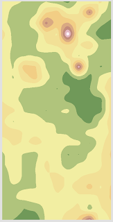
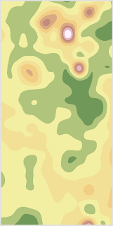
Inverse Distance Weighted or IDW interpolation is a deterministic tool which determines each cell's value by finding the average of nearby cells' values.  Closer cells are 'weighted' in this determination, making near cell values  stronger determinants of an individual cell's value than more distant cells' values.  The ultimate value of the cell in question is the value for that cell which minimizes the root mean square prediction error.



Kriging 1

Kriging 2

 Kriging is a geostatistical interpolation method that uses statistical relationships between values in the determining of each interpolated cell value. In addition to considering the data given, this model uses spatial autocorrelation semivariograms to determine which values are factored into the interpolation of each point.  Simply put, kriging determines weight by looking at each value's relationship to other values in addition to their relationships to the value being found.  For our model, we determined that ordinary kriging with a spherical semivriogram would be most appropriate, as there is no external variable we expect to bias our data in terms of elevation that can be defined by an equation and autocorrelation of elevation decreases substantially with distance.




Natural Neighbor 2

Natural Neighbor 1

        

Natural Neighbor interpolation works by  creating two Voronoi diagrams from the dataset for each cell: one using only nearest data points and one using the cell as an additional point. It then weights each nearest value by the percentage of that value's Voronoi polygon which is overlayed with the interpolated value's polygon.  Simply put, natural neighbor works by weighting each point not only by how close it is, but also how close it is to other points in the same direction from the cell being determined.  Doing this 

Spline 1

Spline 2

   Spline Interpolation develops a smooth mathematical curved plane, the function of which fits each input data point perfectly and therefore produces a continuous surface devoid of artifacts.  It usually does better with surfaces that don't contain coarse variation than with regions of varied elevation, because this model will be warped by concentrated variations in input points.

TIN 1

TIN 2

       Triangular Irregular Netwroks (TINs) are simply digital triangles drawn between nearest data points. Which points are connected by the edge of a triangle are determined such that no vertex lies inside the polygon of another triangle. 

                 Once the rasters were complete, a we determined the most effective interpolation methods for our data to be Kriging and Spline.  3D Elevation models were developed for the five models by importing the rasters (or TINs) into ArcScene and setting the base height to the surface of the elevation values assigned each cell.  After playing around with a little symbology, what we ended up with for our Spline and Kriging models can be seen below. 

Spline

Kriging

Conclusions

                 In my opinion, the Kriging model best represents our data of the five DEMs which we developed. It is the only model which allowed for the mesa which I had hoped to digitize which was surprising to me (in the upper left region you will notice a brown hump with a somewhat flat top). It also contained the best ridge between the large mountain and its northwest neighbor. The Spline model was too smooth, where our terrain was very rough. IDW was a very sperical model which poorly represented the more linear, continuous features such as the aforementioned ridge and the trough (which none of the models performed well with, probably because our sampling method in data collection was poor) and natural neighbors split the difference between IDW and Spline.  Because of our sampling, the TINs were simply too rough, the trinagles too large to be of much value when compared to the raster-based models.

               Our original data collection in both models was very course.  Collecting a higher number of points, especially in areas of greater elevation, would have certainly helped out models achieve greater consistency with our original surfaces.  However, no amount of hand-determined data collection is going to remotely rival the results that are achieved with LIDAR.  As other groups have discussed, the weather was of course a factor involved with our execution of this exercise: in the future our data collection will likely involve a visit to accuweather and a warm pair of gloves.  Professor Hupy suggested that it may be prudent to have the person writing down the data points remain inside and have the information radioed the outside, as to avoid them having to sit there with their writing hand exposed.  Our group had the fortune in both collections to avoid the coldest of the weather during each week; however in cases where we would not be so fortunate, or where we would have to survey something further from the comfort of indoor heating, I would certainly consider that option. In some scenarios, I might have to.

Ultimately, I would think that which DEM works best for one’s purposes depends on what those purposes are. I am personally partial to the Kriging model because I found it’s representation of our data to be the most accurate, but I honestly only have a basic grasp on how it works. Clearly, it would be more effective for data that has some "directional bias," as ESRI puts it, such as a prevailing wind or geologic flow.  Spline is extremely smooth by comparison with even the Natural Neighbor and IDW methods, and may work best for continuous surfaces that don't have extreme values that must be accounted for in the model.  Natural Neighbor and IDW seem to work in very similar ways to one another, being derived from an average of weighted neighbors.

Discussion

                It would have been nice to compare the elevation data from select points on the DEM’s to the original surfaces, but in both surveys our land was destroyed well before we were finished building the models.  It would also have been interesting to take some more precise readings with remote sensing equipment and compare DEM’s developed with those methods to our rudimentary, low-resolution meter-stick method. I also would have liked to have had a grounding in the various interpolation methods used before trying to decide on how to use them.  ArcHelp is wonderful, make no mistake, but spatial interpolation is perhaps a topic in which I could have used a little more priming. In fact, ArcHelp itself mentions in the Kriging page that the process is more complicated than they have the space (or perhaps more appropriately patience) to really get into.

I am lucky to have a group that works well together.  One of our members couldn't be there for the lecture and lab in which we discussed how to make these 3D models happen, but we made it work and all three of us have now used several methods of raster interpolation to create 3D Digital Elevation Models.  We completed the projects relatively quickly and without getting too frustrated, mostly, which when exploring GIS in sandbox mode really says something.